

Recap: Computation and Physical Effects
02: sensing, sampling, and codes. 03: computation, storage, and handoff.
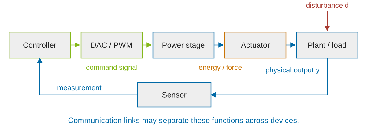
The result must reach the output and cause a timely physical effect.
A Direct Electrical Output
A digital-to-analog converter (DAC) maps a code to an electrical level.

- ADC: voltage → numerical code, already covered in Chapter 02.
- DAC: numerical code → voltage or current representing an output value.
The output level carries a command; a motor needs a power stage.
Circuit Rules for the DAC
Task: add the DAC’s branch currents, then convert their sum to an output voltage.
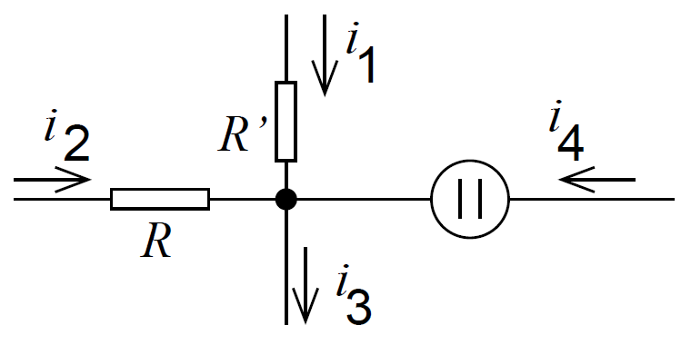
Node: incoming current equals outgoing current.
\[I = I_0+I_1+I_2+I_3\]
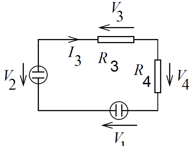
Loop: signed voltage changes sum to zero.
\[\sum_k V_k=0,\qquad V_R=RI\]
Diagrams: Chen / Marwedel, after Jewett and Serway (2007). \(I_i\): branch currents; \(V_k\): signed voltages; \(R\): resistance. Signs follow the chosen arrows.
Op-Amp Feedback and Virtual Ground
Goal: convert the summed current \(I\) to \(V_{out}\) while keeping the summing node near \(0\,\mathrm{V}\).

\[V_{out}=g(V_+-V_-),\qquad I_{in}\approx0,\qquad V_{out}\approx -R_f I\]
\(g\): open-loop gain; \(V_+,V_-\): input voltages; \(R_f\): feedback resistance. Assumptions: negative feedback, linear operation, sufficient output swing. Virtual ground is not a wire to ground.
A Weighted-Resistor DAC
Each switch applies either \(V_{ref}\) or 0 to its resistor branch.

Circuit: Chen / von der Brüggen (2024), based on Marwedel, Fig.3.51. \(x_0\): LSB; \(x_3\): MSB; \(R_1=R_f\) in our equations. Ideal switches and linear op-amp model.
Bits Become Weighted Currents
For bit \(i\in\{0,1,2,3\}\):
\[I_i=\frac{x_iV_{ref}}{2^{3-i}R}\]
At the summing node:
\[I=\sum_{i=0}^{3}I_i=\frac{V_{ref}}{8R}\underbrace{\sum_{i=0}^{3}x_i2^i}_{X}\]
The total current is proportional to the numerical code \(X\).
\(x_i\in\{0,1\}\): bit values; \(X\): unsigned integer 0–15; \(V_{ref}\) [V]; \(R\) [Ω]; \(I_i,I\) [A]. Virtual-ground and ideal-switch assumptions apply.
Current Becomes Output Voltage
\[V_{out}=-R_f I=-V_{ref}\frac{R_f}{8R}X\]
With \(R_f=R/2\) and \(V_{ref}=3.2\,\mathrm{V}\):
| Code | Integer \(X\) | Output |
|---|---|---|
| 0000 | 0 | \(0\,\mathrm{V}\) |
| 1000 | 8 | \(-1.6\,\mathrm{V}\) |
| 1010 | 10 | \(-2.0\,\mathrm{V}\) |
| 1111 | 15 | \(-3.0\,\mathrm{V}\) |
One code step changes the output by \(-0.2\,\mathrm{V}\) in this circuit.
Chosen ideal example: adequate negative supply and output swing. Sign and scaling are circuit-specific.
Pulse-Width Modulation
PWM encodes a value in the fraction of each period spent HIGH.

\[D=\frac{t_{HIGH}}{T_{PWM}}\]
For an ideal \(0/V_H\) pulse signal:
\[\overline{v}=D\,V_H\]
- PWM + low-pass filter: approximate an analog output from the duty cycle.
- Carrier ripple, useful bandwidth, and filter delay constrain the result.
Figure: Marwedel (2021), Fig.3.59, p.187. \(D\): duty cycle; \(t_{HIGH},T_{PWM}\) [s]; \(V_H,\overline v\) [V]. Average voltage does not imply motor speed proportional to duty cycle.
PWM Hardware and Resolution
Goal: generate programmable PWM pulses without software timing each edge.
Counter: \(k=0,\ldots,N-1\).
Source comparator: HIGH if \(k>r\).
\[f_{PWM}=\frac{f_{clk}}{N},\quad D=\frac{N-1-r}{N}\]
With \(f_{clk}=20\,\mathrm{MHz}\), \(N=1000\):
- \(f_{PWM}=20\,\mathrm{kHz}\)
- Duty step: \(1/N=0.1\%\)
- \(r=749\): 250 HIGH ticks (\(25\%\))

Figure: Marwedel (2021), Fig.3.60, p.188; power stages omitted in its schematic. \(f_{clk}\) [Hz]: timer clock; \(N\): ticks per period; \(r\): compare register. Chosen strict-\(>\) model; endpoint conventions and update latching vary by timer.
The DAC Hold Output
Unlike the PWM pulse train, a DAC keeps each level until its next update: zero-order hold (ZOH).

Original plot: P. Marwedel, via Chen / von der Brüggen (2024). Dashed: source signal; solid: held output. Ideal vertical steps omit settling time. Time axis follows the original example.
One Sample and Its Sinc Contribution
Problem: interpolate between samples while preserving every sample value.

Solution: a shifted sinc has weight 1 at its own sample, 0 at the others.
Original plot: P. Marwedel, via Chen / von der Brüggen (2024). Horizontal coordinate: \((t-sT_s)/T_s\); vertical: interpolation weight. Between sample instants, neighboring samples contribute.
Contributions of Several Samples
Each colored curve is one weighted, shifted sinc; add their values at the same time.

Original plot: P. Marwedel, via Chen / von der Brüggen (2024). Staircase: held samples. Colored oscillating curves: individual interpolation terms, not successive output states.
Reconstruction and Remaining Error
The finite sinc sum follows the signal more closely than the held staircase.

Original plot: P. Marwedel, via Chen / von der Brüggen (2024). Blue: original; green: held samples; red: finite reconstruction. Quantization and omitted contributions prevent an exact match here.
Input and Output Filters
Goal: reconstruct the original signal with minimal error.

| Stage | Problem | Approach |
|---|---|---|
| Input: anti-aliasing | Out-of-band content aliases. | Limit analog bandwidth before sampling. |
| Output: reconstruction | Conversion adds spectral images; the hold distorts the useful band. | Low-pass filter; compensate hold distortion where needed. |
An output filter removes spectral images, but cannot undo aliasing or quantization.
Communication Within and Between Devices

Topology, electrical conditions, traffic, and timing requirements guide the choice.
SPI Transactions
SCLK clocks bits; CS selects the target. Data can flow in both directions.

Example: CPOL=0, CPHA=0. MOSI/MISO names describe directions relative to the controller. Timing: Analog Devices AN-1248. SPI formats, CS timing, modes, and integrity checks depend on the device.
I²C Transactions
Two shared signal lines: SDA for data, SCL for clock.

S/Sr/P: START / repeated START / STOP; A/N: ACK / NACK. Example: 7-bit addressing, one register byte, two data bytes. NXP UM10204 Rev.7.0, §3.1. Clock stretching may extend SCL LOW.
Bus Clocks and Application Timing
An OS can run other tasks while this caller waits for HW.
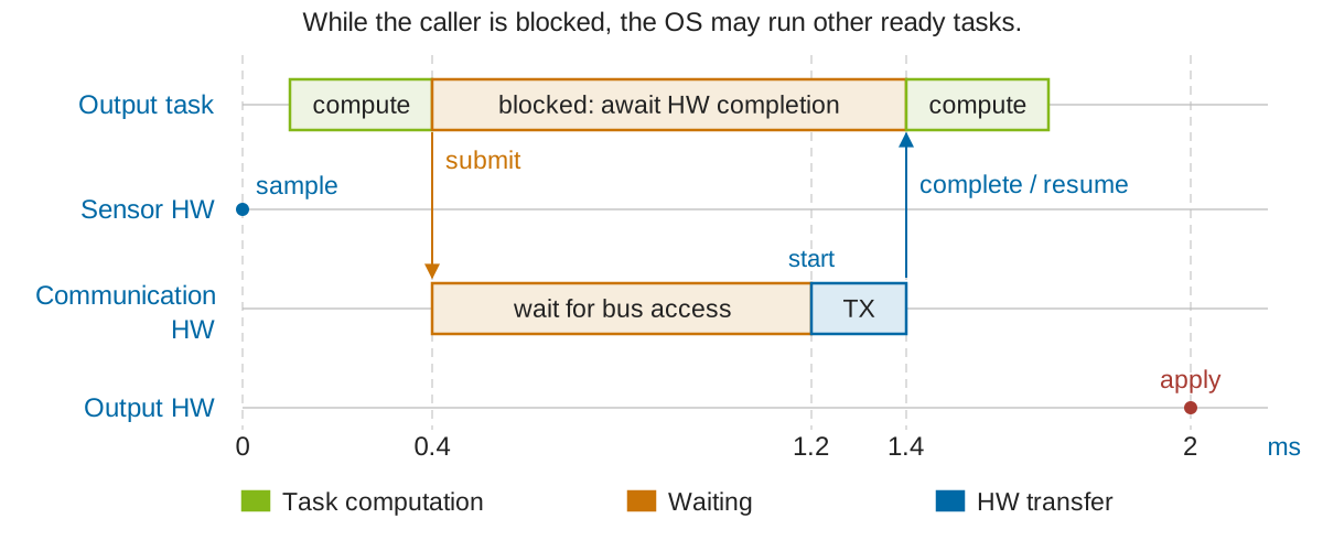
Interrupts/DMA can hide HW latency with useful computation.
Example: immediate resumption at completion; transfer \(0.2\,\mathrm{ms}\), sample age \(2.0\,\mathrm{ms}\). Latency hiding improves CPU use; it does not shorten the transfer or guarantee a fresher output.
Differential Signaling

Single-ended: compare a signal with its reference ground.
Differential: compare the two wire voltages:
\[V_D=V_A-V_B\]
Common disturbance \(n\):
\[(V_A+n)-(V_B+n)=V_D\]
Limits: common-mode range, matching, thresholds, and termination.
Figures: Marwedel (2021), Figs.3.47/3.48. \(V_A,V_B,n\) [V]; \(V_D\): differential voltage. Differential signaling does not inherently require negative supply voltages; real receivers reject common-mode interference only within limits.
CAN: A Shared Embedded Bus
CAN broadcasts frames; identifiers express message content and arbitration priority.

- Bit timing must accommodate propagation and transceiver delays.
- Higher bit rates generally tighten the permitted physical timing budget.
Generic high-speed CAN. ECU: Electronic Control Unit. Physical-layer and configuration limits constrain nodes, length, stubs, and termination.
CAN Arbitration Bit by Bit
0 is dominant; 1 is recessive. A node sending 1 stops when it reads 0.

Rows show intended identifiers, most significant bit first. Bit 1 is the second bit from the right. Example: two Classical CAN standard data frames; no higher traffic or errors shown.
CAN Frames and Error Handling

- Classical CAN: 0–8 data bytes; 15-bit CRC sequence.
- ACK: at least one receiver accepted the frame at link level.
- Detected errors may trigger retransmission; error counters can restrict a node.
- CAN FD: up to 64 data bytes, changed CRC rules, optional faster data phase.
Standard data-frame schematic, not proportional bit timing. Arbitration: 11-bit ID + RTR; Control: IDE + reserved bit + 4-bit DLC. Stuff bits add overhead. ACK does not confirm application acceptance or actuator effect. Bosch M_CAN Rev.3.3.1, §3.1.
Priority and Non-Preemptive Blocking
Even the highest-priority ready frame waits for a frame already in progress.
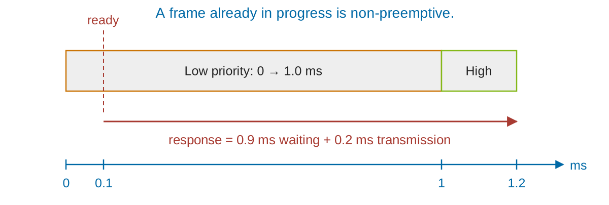
Other priorities can also have bounds when traffic, frame sizes, and errors are bounded.
Illustrative timing model: one ongoing frame, one new high-priority frame, no further traffic/errors. Response time starts at readiness. Formal CAN response-time analysis is later material.
TDMA Time Windows
Time Division Multiple Access: each participant transmits in assigned windows.

- A shared time basis coordinates slot boundaries.
- Guard time accommodates bounded clock/timing uncertainty.
- Slots reserve service even when another participant has more traffic.
Figure: Marwedel (2021), Fig.3.49, p.176. Based on the TDMA discussion cited by Chen, including E. Wandeler and L. Thiele, ASP-DAC 2006. Fixed slots are the model here; variants need their own bounds.
Waiting for the Next TDMA Slot

Model: \(P=10\,\mathrm{ms}\), one \(2\,\mathrm{ms}\) slot, transmission \(C=1\,\mathrm{ms}\).
\[W<P,\qquad R=W+C<P+C=11\,\mathrm{ms}\]
\(P\): cycle period; \(C\): transmission duration; \(W\): access wait; \(R\): readiness-to-completion time. Start only at slot boundary; frame fits with required reserves; next start is usable; bounded synchronization error; no faults.
FlexRay Communication Cycle

- Static slots reserve time; used dynamic slots extend beyond a minislot.
- Two channels support redundancy; a guardian can enforce transmit windows.
Cycle excerpt: Chen / Marwedel, via TZM FlexRay Introduction. A1/B1/etc. label messages from nodes A/B/etc. A guardian is an additional mechanism; channel redundancy does not remove every common cause of failure.
Switched Ethernet and TSN
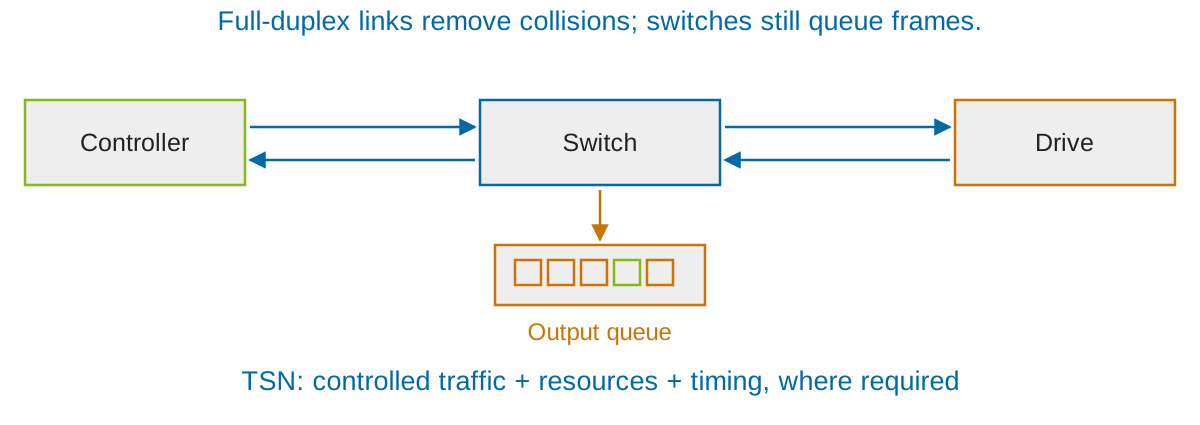
- Full duplex uses point-to-point links without CSMA/CD collisions.
- Queues, competing streams, and forwarding still affect delay.
- TSN combines mechanisms for bounded latency, timing, and resource control.
IEEE 802.3 full-duplex operation; IEEE 802.1 Time-Sensitive Networking. A TSN-capable device alone does not establish an end-to-end bound: topology, configuration, traffic assumptions, and the selected mechanisms matter.
Output Signals and Actuation Power


- The command carries information.
- The power stage switches or amplifies energy from a supply.
- The actuator applies torque or force to the load.
- Displays are another output path, with different physical requirements.
Motor photo: P. Marwedel, via Chen / von der Brüggen (2024). Diagram: generic motor drive.
Actuator Dynamics
A command update may precede its physical effect by a substantial interval.
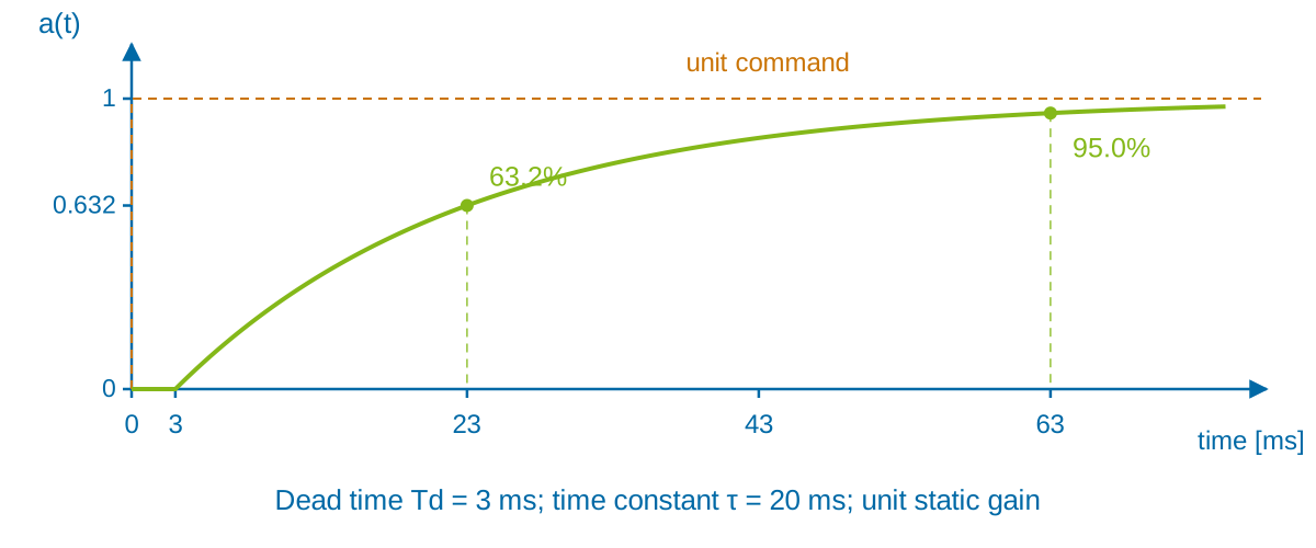
Illustrative model: \(a(t)=0\) for \(t<T_d\); then \(a(t)=1-e^{-(t-T_d)/\tau}\). \(a\): normalized actuation; \(T_d=3\) ms; \(\tau=20\) ms. Not measured motor data. Saturation and rate limits require additional modeling.
The Plant Input and Feedback

\[\dot{x}=f(x,a,d),\qquad y=h(x)\]
\(u_{cmd}\): intended command; \(a\): actual actuation entering the plant; \(d\): disturbance; \(x\): plant state; \(y\): physical output; \(y_m\): measurement. Known commands support prediction; measurements correct state estimates. The actuator may alternatively be included inside the plant model.
Missing or Stale Commands
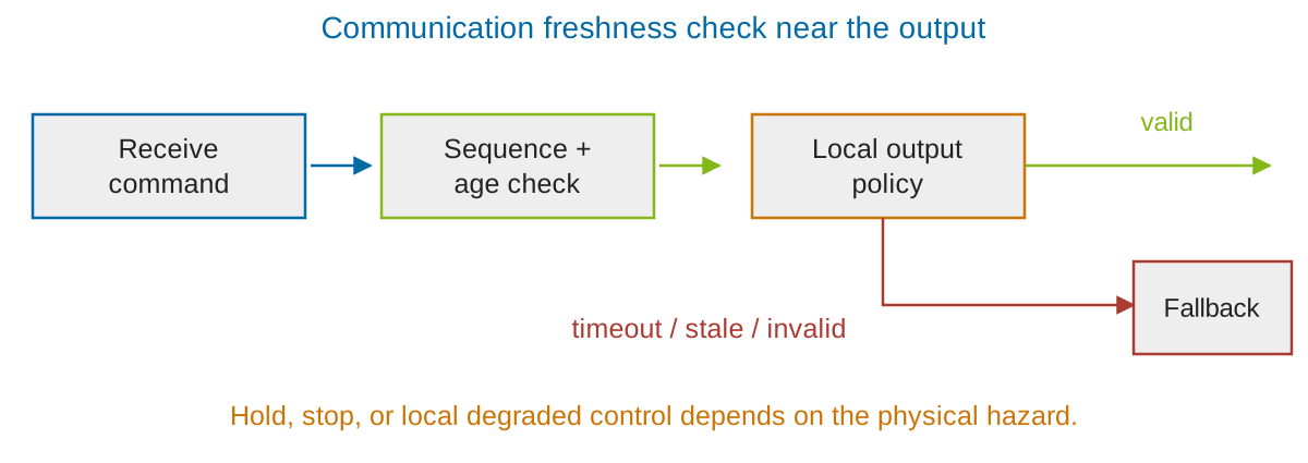
- Detect missing updates and invalid or stale commands locally.
- Choose hold, controlled stop, or degraded operation from the application needs.
- Monitor the physical effect where command receipt alone is insufficient.
A communications timeout is a detection mechanism. The appropriate output response depends on plant dynamics, stored energy, and the fault model; “keep last value” and “switch off” are not universal safe states.
Voting Before and At the Actuator
Several actuation channels act on a common mechanical output.

Conceptual three-channel comparison, not a Shuttle schematic. Historical example: J. E. Tomayko, NASA-CR-182505 (1988), Ch.4.4: the Shuttle used quadruple redundant actuation with physical voting. Fault assumptions, common causes, and mechanical coupling remain decisive.
End-to-End Timing and Physical Response
Sample age: \(A_{apply}=t_{apply}-t_{sample}=2.0\,\mathrm{ms}\).
The \(1.5\,\mathrm{ms}\) application deadline is missed despite a \(0.2\,\mathrm{ms}\) transfer.
\(A_{apply}\): sample age when the output applies its derived command. Actuator/plant response follows application and must be assessed separately. Bounds on individual stages compose only when their assumptions and event definitions are compatible.