Embedded Hardware Fundamentals
Embedded Systems / Cyber-Physical System Fundamentals (ES/CPSF)


The Hardware Loop
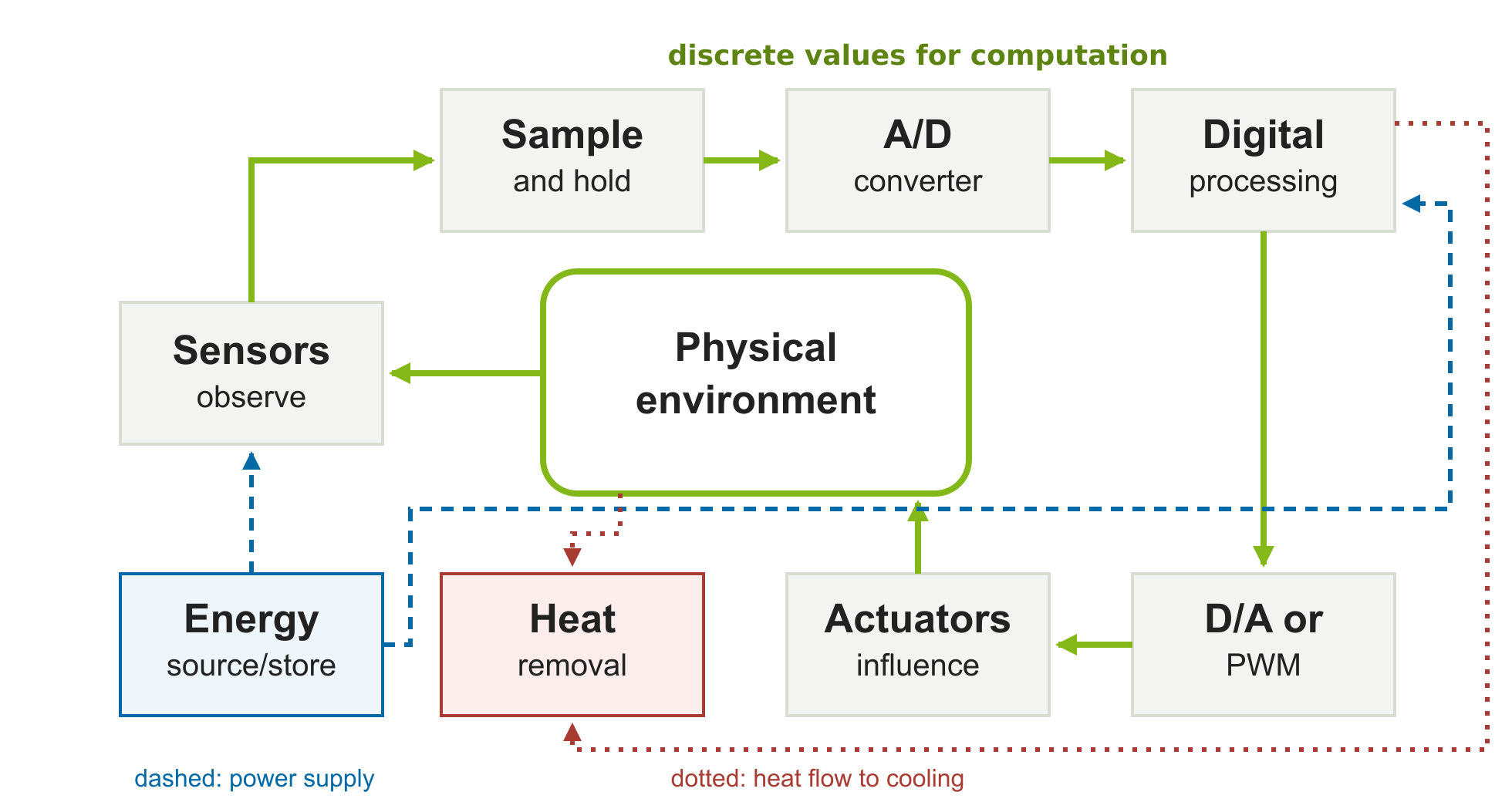
Hardware loop after Marwedel / Chen. Solid green: signal/control flow; dashed blue: power supply; dotted red: heat removal.
Sensors: Emergency Braking Assistance
An emergency braking assistant must detect an obstacle early enough to react.
- Radar: distance and relative velocity from reflected radio waves.
- Camera: image data for object and lane recognition.
- Wheel sensors: motion estimates from magnetic or optical effects.
A sensor converts a physical quantity into an electrical signal; software interprets that signal.
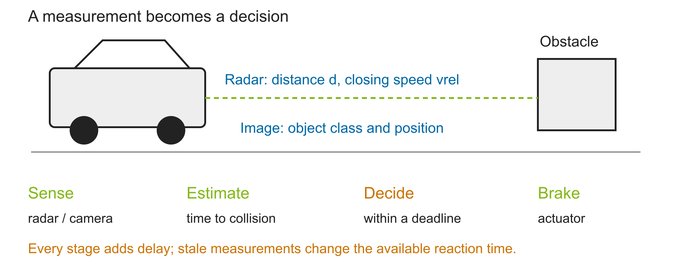
Distance alone is not enough: measurement age, uncertainty, and relative speed affect the decision.
Simplified teaching example, not a production braking algorithm. EBA: emergency braking assistance.
Sensor Families
Motion
Acceleration and angular rate for navigation, balance, and control.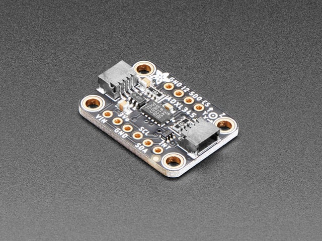
Optical
Light intensity and images for perception and measurement.Identification
RFID and biometrics connect physical identity to digital decisions.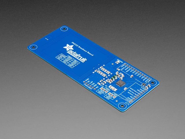
Environment
Pressure, temperature, and chemistry expose operating conditions.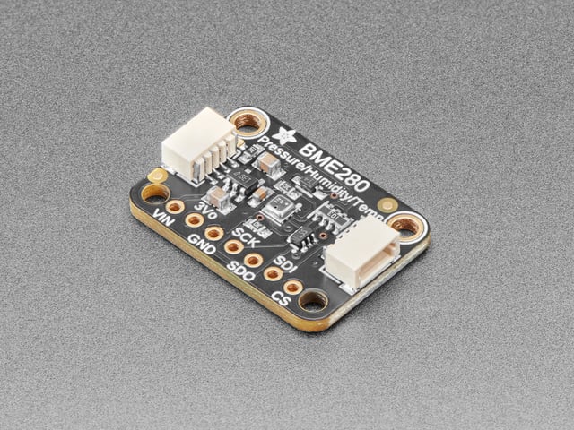
Automotive
Position, speed, and pressure support engine and safety functions.Smart sensors
Integrated logic preprocesses data close to its physical source.Rain Sensors
Infrared light enters the windshield at about 45 degrees.
- Dry glass returns much of the light by internal reflection.
- Water changes the optical boundary: less light reaches the receiver.
- The wiper controller reacts to the measured intensity.
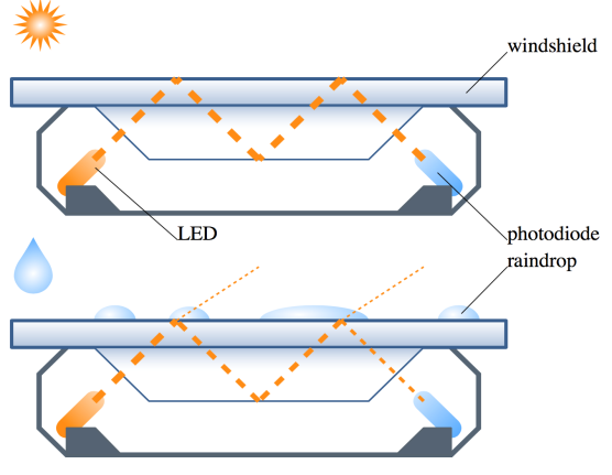
A physical effect becomes a measurement without directly measuring water volume.
Chen / Marwedel 2024, Inputs p.8.
CCD Image Sensors
Photons create charge packets in pixel cells.
- Clocked gates transfer charge to the next cell.
- Sequential transfer brings charge to the readout amplifier.
- Readout and A/D conversion produce image data.
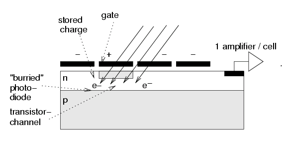
The measured value is physically transported before it becomes a digital number.
Chen / Marwedel 2024, Inputs p.9.
CMOS Image Sensors
Standard CMOS production allows pixel circuitry and logic on one chip.
- Row/column addressing selects pixels.
- Amplifiers, multiplexers, and ADCs provide readout.
- Timing, interface logic, and preprocessing can be integrated.
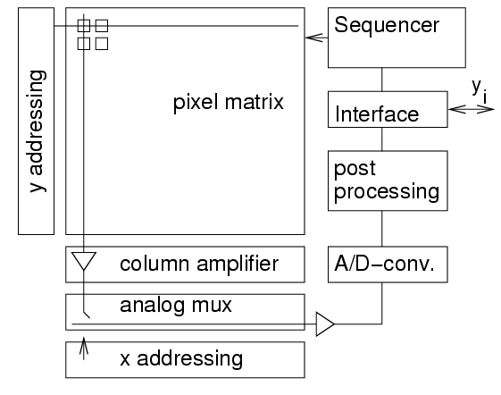
Memory-like access and integration distinguish CMOS readout from serial CCD charge transfer.
Chen / Marwedel 2024, Inputs p.10.
Biometrical Sensors
Fingerprint sensors acquire a physical surface pattern using optical, capacitive, or thermal effects.
- Matching thresholds trade false acceptance against false rejection.
- Calibration, contamination, aging, and spoofing affect the system.
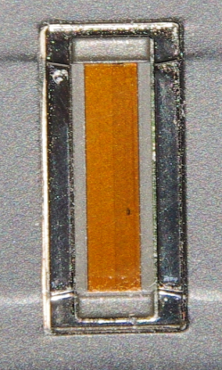
Sensor acquisition and the identity decision are separate parts of the system.
Fingerprint sensor photograph: Marwedel 2010 / Chen Inputs p.12.
PAMONO: An Embedded Monitoring Pipeline
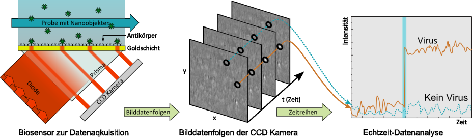
Binding at a coated surface → CCD image sequence → real-time detection.
The embedded challenge: distinguish small optical changes from artifacts within limited time, computing capacity, and energy. Monitoring does not require an actuator.
Figure: Chen Inputs p.13 (labelled “PAMANO”); project name: PAMONO. ISAS: optical detection and resource-optimized real-time analysis, 2020.
Signal Domains
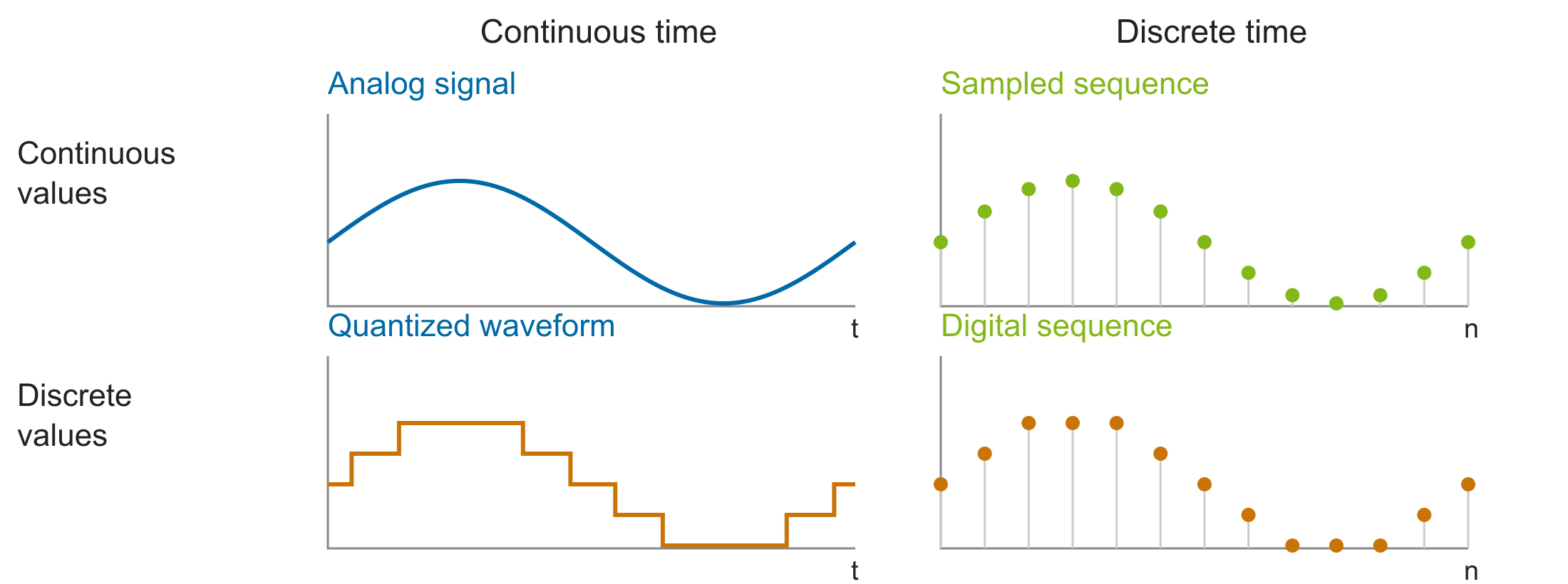
A signal maps time to values: \(s:D_T\rightarrow D_V\). Sampling discretizes time; quantization discretizes values.
Sample-and-Hold Circuits
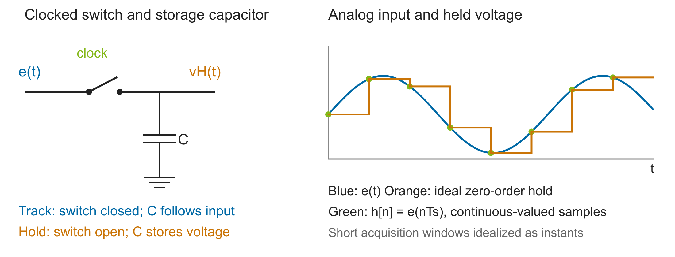
\(h[n]=e(nT_s)\) is a discrete-time sequence; the capacitor output remains an analog voltage held for conversion.
Track: charge and settle. Hold: keep the input stable while the ADC determines its code.
Fourier Approximation: K=1 and K=3
The target is the square wave in both plots. We build it as a sum of sine waves, beginning with the fundamental.
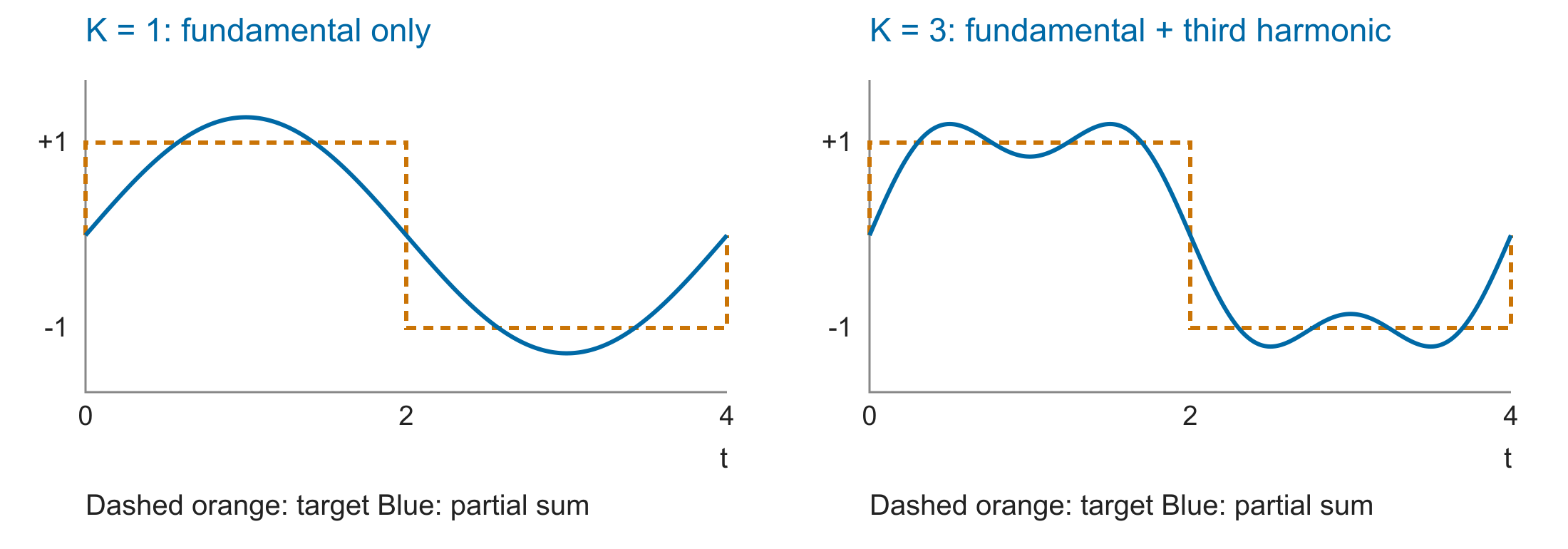
Left: only \(k=1\). Right: add \(k=3\) with one third of the amplitude. The sum starts to resemble the same target square wave.
Fourier Approximation: K=5 and K=7
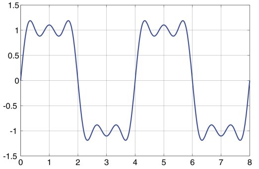
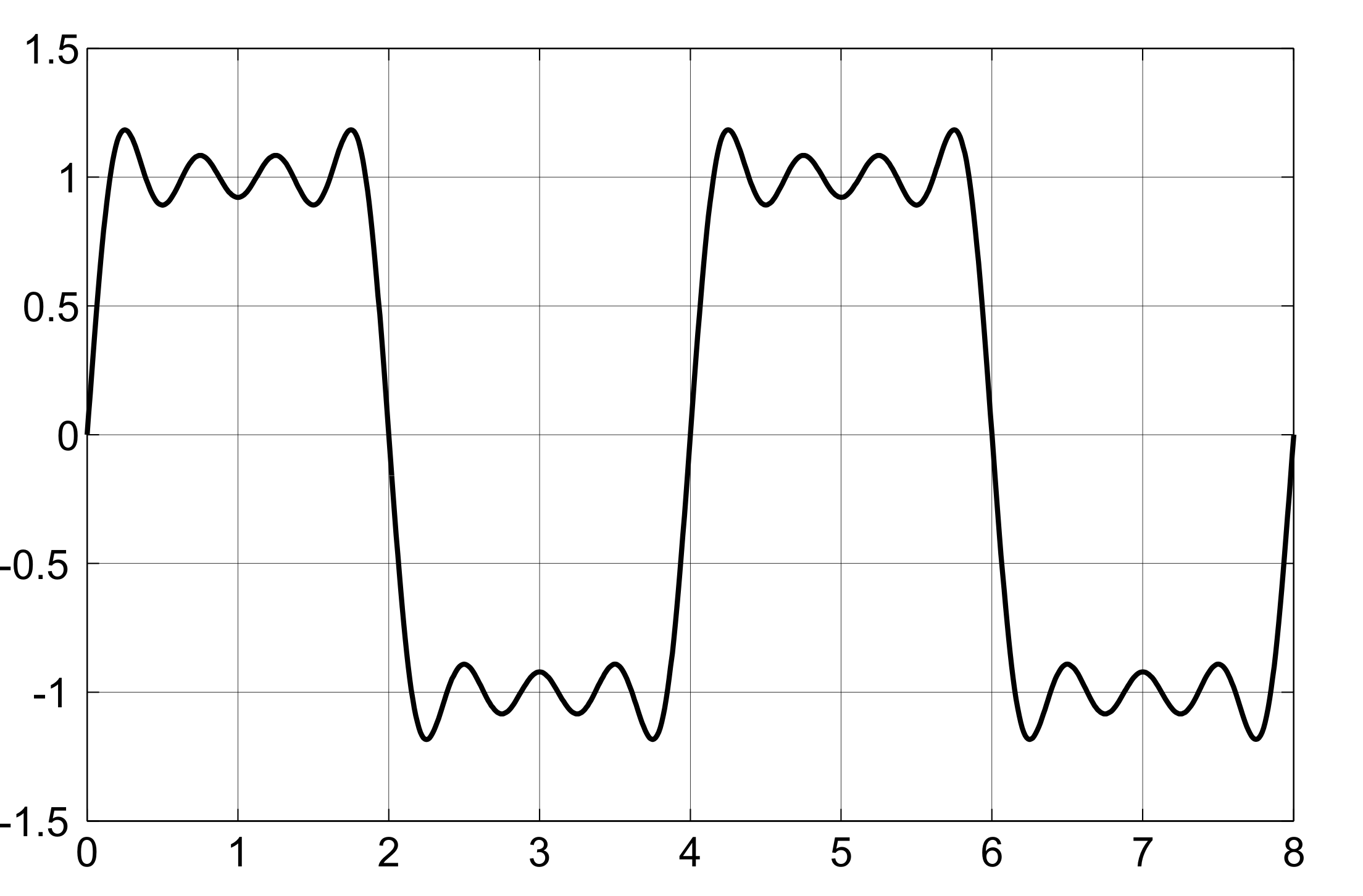
Chen / Marwedel 2024, Inputs, PDF p.20; original PowerPoint image.
Fourier Approximation: K=9 and K=11
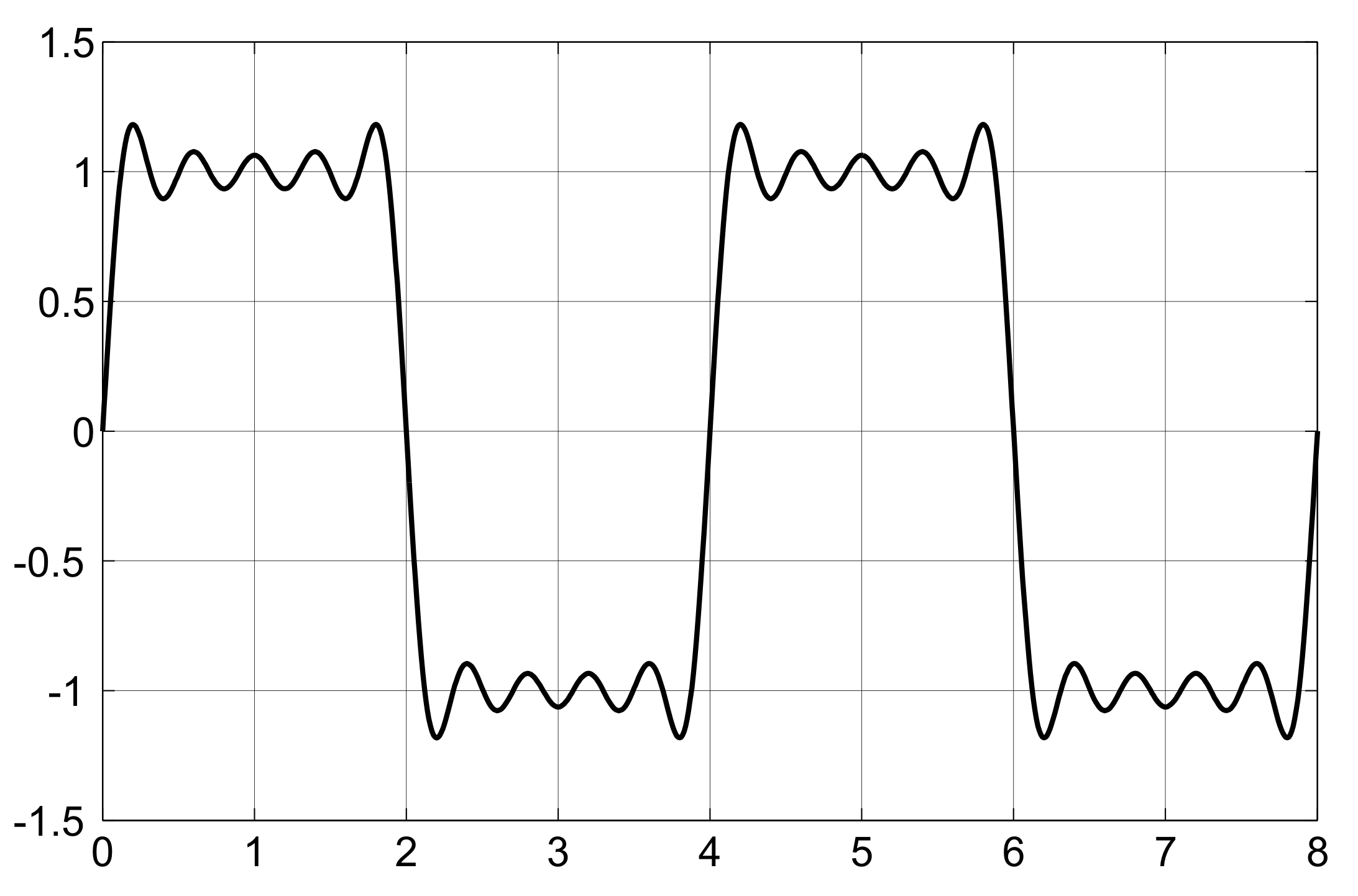
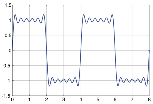
Chen / Marwedel 2024, Inputs, PDF p.21; original PowerPoint image.
Aliasing
The obstacle to reconstruction: different continuous signals can give identical samples.
\[e_3(t)=\sin(2\pi t/8)+0.5\sin(2\pi t/4)\] \[e_4(t)=e_3(t)+0.5\sin(2\pi t)\]
At integer times \(t=n\), \(\sin(2\pi n)=0\): both continuous signals give the same samples.
Plot: solid \(e_3\), dashed \(e_4\); the integer times are the sampling instants.
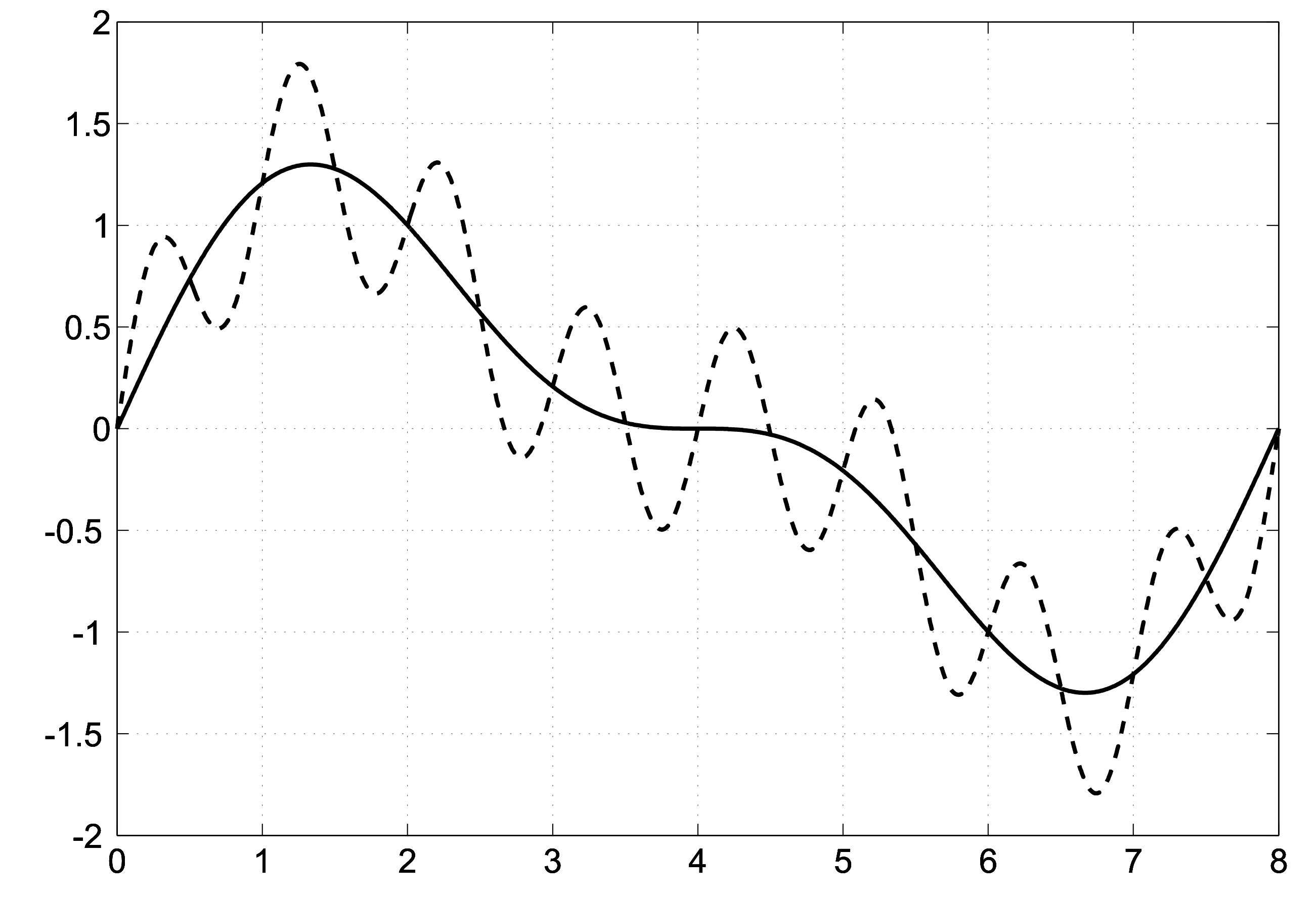
The added 1 Hz component disappears at \(f_s=1\) Hz. Without a bandwidth limit, reconstruction is not unique.
\(t\): time in seconds; \(n\): integer sample index; \(e_3,e_4\): continuous-time signals. \(f_s=1/T_s\): sampling rate; \(T_s\): sampling period. \(f_{max}\): highest input frequency (1 Hz for \(e_4\) here); \(f_s/2\): Nyquist limit.
Sampling Theorem: Exact Recovery Is Possible
\[f_s > 2f_{max}\]
A signal with no components above \(f_{max}\) can be reconstructed exactly from its ideal, uniformly spaced samples. \(f_s/2\) is the Nyquist limit.
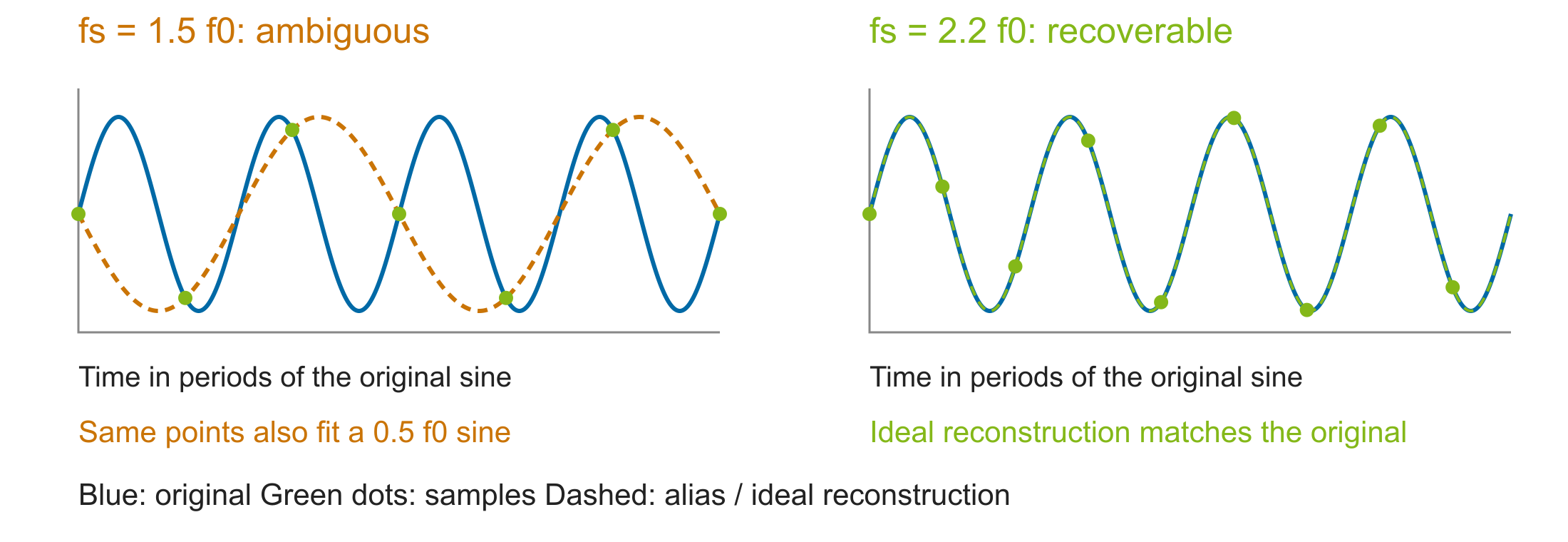
\(f_s\): sampling rate; \(f_{max}\): highest input frequency; \(f_0\): sine frequency in the plots. Ideal reconstruction uses the complete sample sequence, not straight-line interpolation. Here \(f_{max}=f_0\); practical filters require margin.
Anti-Aliasing Filters
The analog filter precedes sample-and-hold:
\(e(t)\rightarrow g(t)\rightarrow h[n]\).
- Ideal: remove frequencies at and above \(f_s/2\).
- Realizable: finite transition band and imperfect attenuation require margin below \(f_s/2\).
- A later digital filter cannot undo frequencies already aliased.
Without the analog filter, components above \(f_s/2\) violate the theorem’s bandwidth assumption and fold into the useful band.
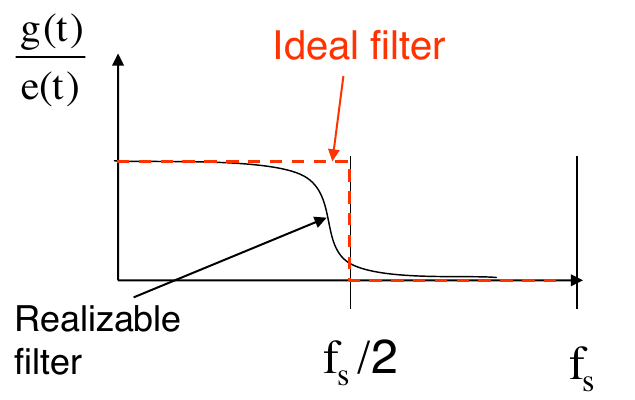
Sensor bandwidth, filter response, and sampling rate must be designed together.
Chen / Marwedel 2024, Inputs p.25.
Aliasing in Images
The same theorem applies in space: pixels are samples. Fine structures above half the spatial sampling rate violate the bandwidth condition and appear as false coarse patterns.
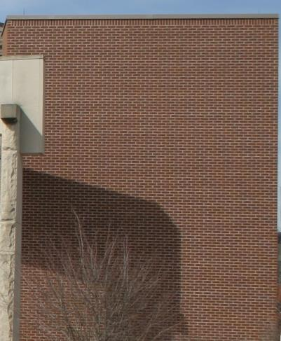
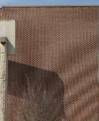
Left: original. Right: subsampled without filtering. Camera and rendering pipelines also need anti-aliasing.
Chen / Marwedel 2024, Inputs p.26.
Successive Approximation
SAR is a common microcontroller ADC architecture: one comparator is reused for a binary search, from MSB to LSB.
- Set the next trial bit; the DAC generates a reference voltage.
- Compare the reference with the held input.
- Keep or clear the bit, then continue.
For \(n=2^b\) levels: \(b=\log_2 n\) rounds. The input must remain held while the DAC and comparator settle at each step.
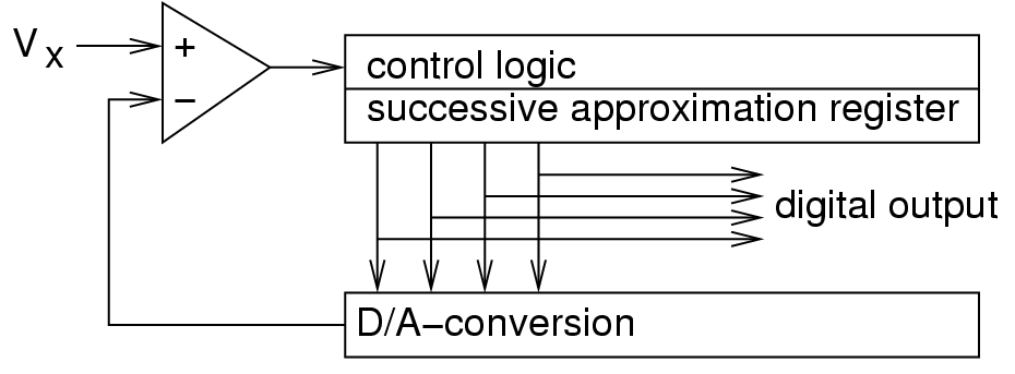
Start with the embedded default: moderate speed, useful resolution, and low power. Flash trades much more hardware for faster conversion.
Chen / Marwedel 2024, Inputs p.32.
Successive Approximation Example
Four-bit example: \(V_{in}=0.70V_{FSR}\); trial voltage \(code/16\cdot V_{FSR}\).
| Trial | Full scale | Decision |
|---|---|---|
| 1000 | 0.5000 | keep bit 3 |
| 1100 | 0.7500 | clear bit 2 |
| 1010 | 0.6250 | keep bit 1 |
| 1011 | 0.6875 | keep bit 0 |
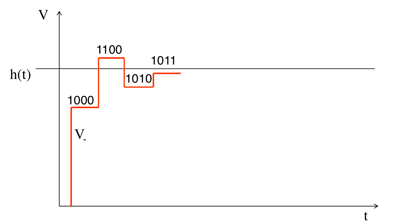
Four sequential comparisons resolve the interval.
Chen / Marwedel 2024, Inputs p.33; native worked example uses the same decision sequence.
Flash A/D Converter
Can we replace SAR’s sequential decisions with parallel comparisons?
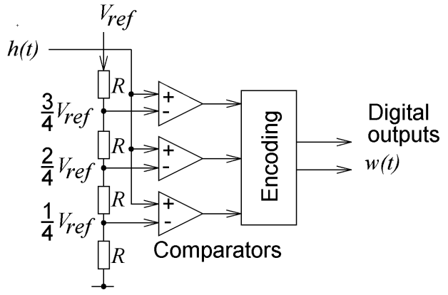
| Input interval | Comparator pattern | Encoded output |
|---|---|---|
| \(0 \le V_{in} < V_1\) | none active | 00 |
| \(V_1 \le V_{in} < V_2\) | lowest active | 01 |
| \(V_2 \le V_{in} < V_3\) | two active | 10 |
| \(V_3 \le V_{in}\) | three active | 11 |
One parallel threshold comparison, then encoding: \(2^b-1\) comparators. Shorter conversion, but more area and power; acquisition and input settling still take time.
ADC Bandwidth and Effective Resolution
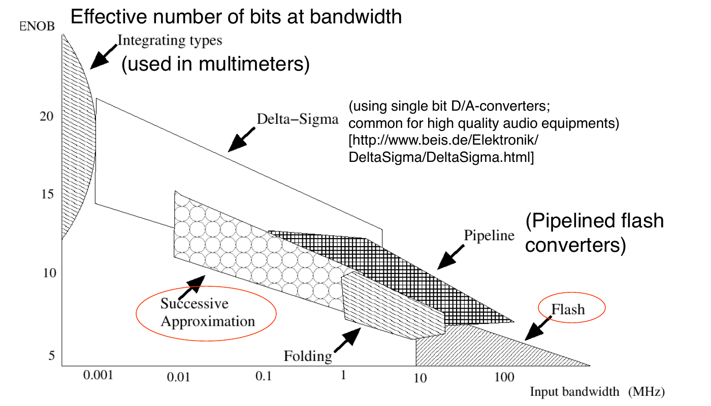
Pipeline: coarse conversion → DAC subtraction → amplified residue to the next stage. Stages work on different samples at once: high throughput, but pipeline latency.
Folding: a nonlinear stage folds the input into a smaller range; decision bits retain which branch was taken. The folded residue is processed further, avoiding a full flash comparator bank.
Application map: Chen / Marwedel, 2024, Hardware Inputs, p.34. ENOB is effective resolution, not merely output-code width.
Quantization Noise
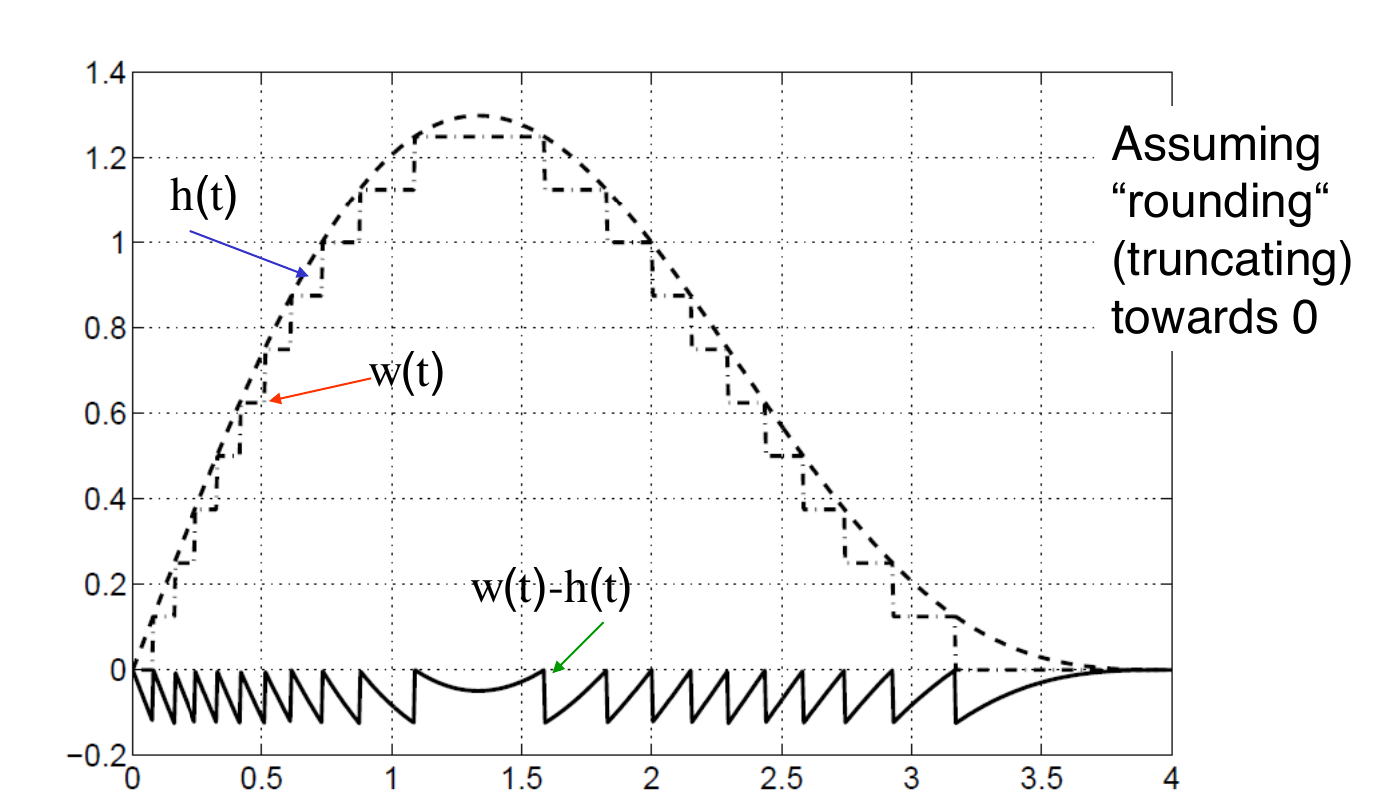
For quantization error \(q=w-h\): rounding gives \(|q|\leq Q/2\) within range. Truncation toward zero has a sign-dependent bias and \(|q|<Q\).
More bits reduce the step size. More speed often costs power, area, or resolution.
Chen Inputs p.35 shows truncation toward zero, not nearest-value rounding.
Code-Size Efficiency
Larger code memories raise cost and fetch energy.
- Store a compressed encoding and decompress on fetch.
- The decoder must be fast, simple, and energy-efficient.
- Compiler, assembler, and hardware must agree on the encoding.
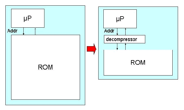
Code density changes the memory system as well as the processor.
Chen Processing p.5.
ARM Thumb as Code-Size Technique
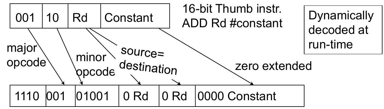
Classic Thumb encodes instructions in 16 bits. An immediate ADD reuses the destination as source; decoding expands opcode/register fields and zero-extends the constant.
Reported for classic Thumb: 65-70% code size, 130% performance with 8/16-bit memory, 85% with 32-bit memory, relative to full-width ARM.
ARM / Gupta via Chen Processing p.6; implementation-dependent results, not a general claim for current ARM cores.
Dictionary: Two-Level Instruction Fetch
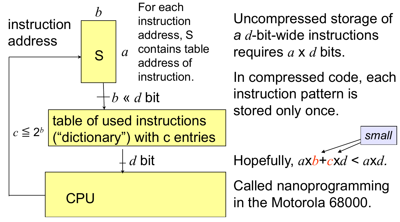
Chen / Marwedel 2024, Processing, PDF p.8.
DSP Filtering as Architecture Driver
Each input sample triggers \(N\) multiply-accumulate operations (MACs). DSP hardware combines multiplication, accumulation, and address updates.
\[x_s=\sum_{k=0}^{N-1}a_k w_{s-k}\]
At sample rate \(f_s\), the filter needs \(Nf_s\) MACs/s. With no buffering, its worst-case processing time must fit within \(T_s=1/f_s\).
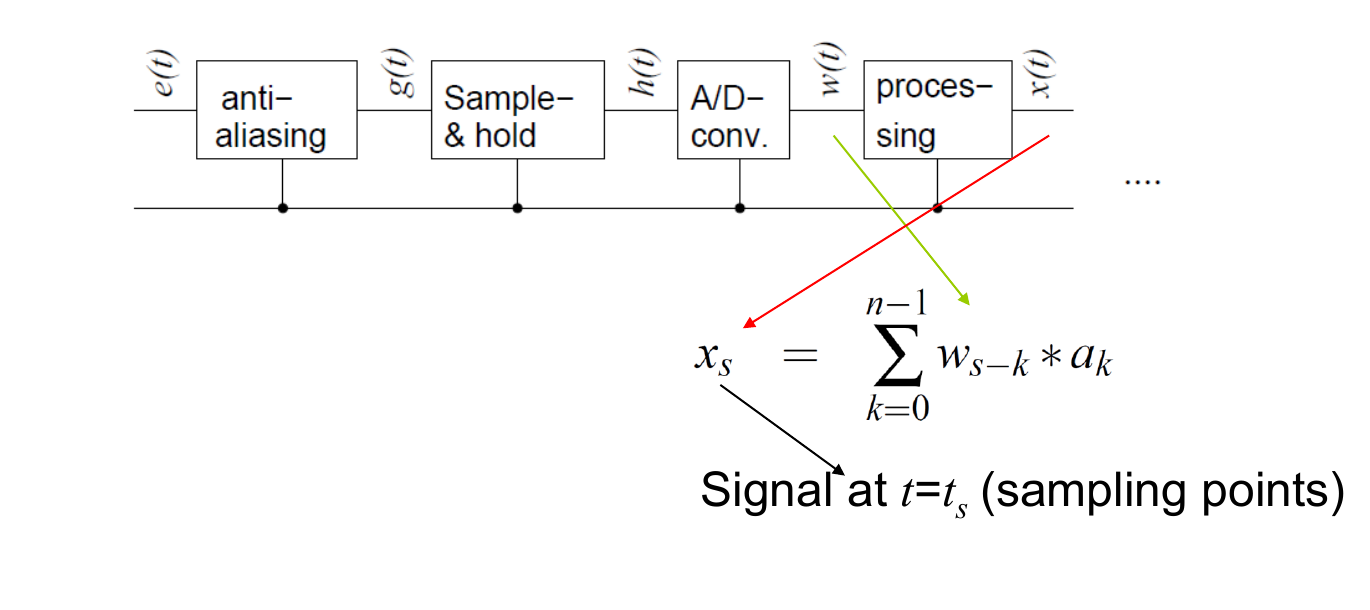
\(w_s\): input samples; \(x_s\): output; \(a_k\): coefficients, newest to oldest sample; \(N\): number of taps; \(s\): sample index; \(k\): tap index; \(f_s\): sample rate; \(T_s\): sample period. Source: Marwedel (2021), Chapter 3.3.2, pp.150-152; Chen Processing p.9.
Fixed-Point Arithmetic
With \(f\) fractional bits, stored integer \(X\) represents \(x=X2^{-f}\).
For a signed word, \(w=1+i+f\): sign, integer, and fractional fields.
In the diagram, \(iwl=1+i\) includes the sign bit, and \(fwl=f\).
- Multiply: \(Z=(X\cdot Y)\gg f\).
- Divide: \(Z=(X\ll f)/Y\).
- Use wide intermediates; check overflow, rounding, and division by zero.
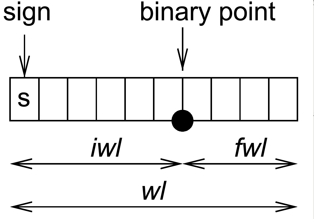
Shifts restore the binary point; they cannot recover already lost information.
Chen Processing PDF p.13, printed slide 14.
Energy and Power
Power \(P(t)\) is measured in watts. Energy \(E=\int P(t)\,dt\), measured in joules, is the area under the power curve over the execution time \(t\).
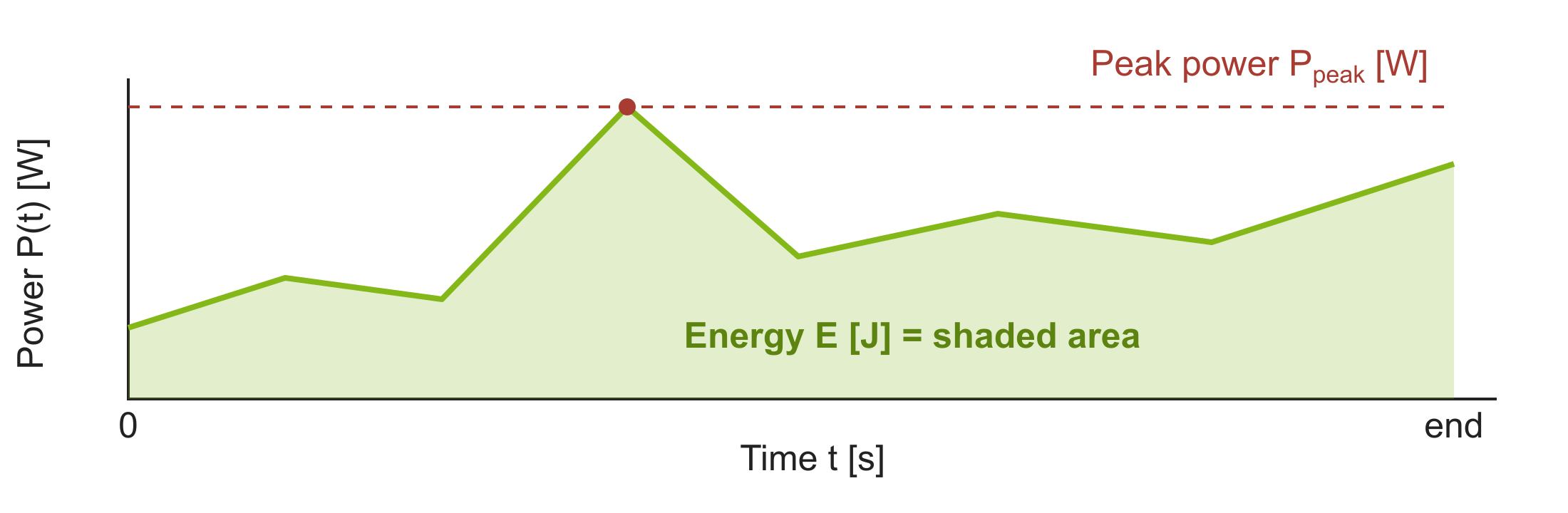
Peak power \(P_{peak}\) affects supply sizing; energy \(E\) affects battery life. Lower power \(P\) can still mean higher energy \(E\) if runtime increases enough.
Power Density and Cooling Pressure
Power density \(P/A\) measures heat generation per chip area \(A\). Cooling limits sustained power \(P\), especially in sealed or passively cooled products.
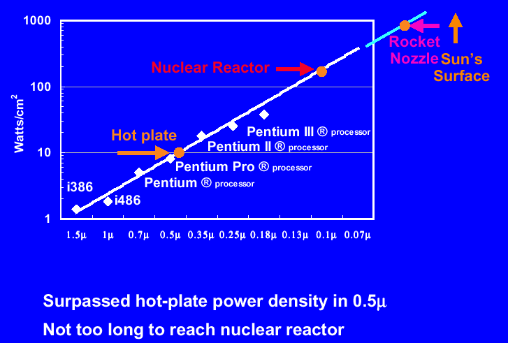
Intel / Pollack via Chen Processing PDF p.16. Logarithmic vertical axis: \(P/A\) in W/cm². The graphic illustrates a scaling concern, not a current forecast. Prescott (90 nm, 2004): about 90 W/cm².
Simpler Cores and Cooling
More complex cores can increase chip area and power \(P\) faster than performance. The chart compares relative gains in area, performance, and performance per watt.
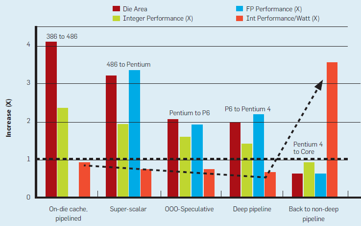
Borkar / Chien, CACM 2011; Chen Processing p.20. Vertical axis: multiplicative increase (1 = unchanged); each group compares successive processor generations. More elaborate cooling adds cost, volume, and energy demand.
Mobile Performance and Power
The chart spans 2G (1995) to 4G (2015).
- Richer codecs, graphics, and radio protocols increase compute and memory demands.
- Workload rises by orders of magnitude on the logarithmic MOPS scale.
- Sustained power remains limited by enclosure, cooling, and battery.
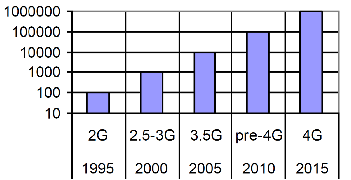
Useful performance per joule matters alongside responsiveness.
Van Berkel, DATE 2009; later years in this source are projections.
Mobile Power Breakdown (2005)
| Component | Share |
|---|---|
| RF modem / amplifier | 30% |
| Application processor | 20% |
| Memories | 20% |
| Display / backlight | 10% |
| Audio codec / amplifier | 10% |
| Other peripherals | 10% |
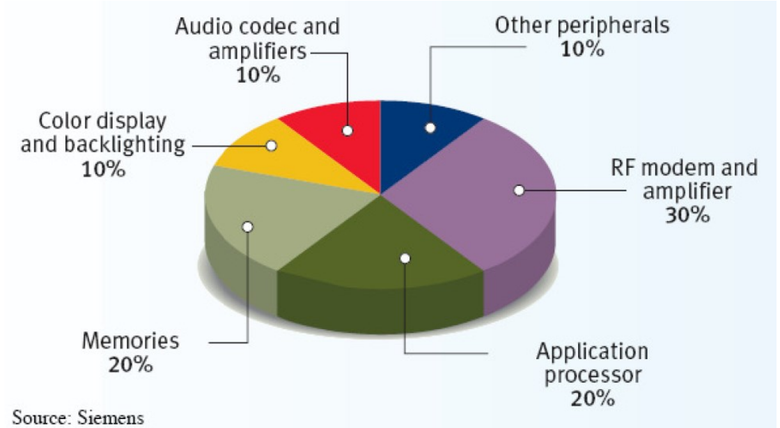
Optimizing only the CPU leaves major platform consumers untouched.
Siemens / Vargas 2005; not a current phone profile.
CMOS Power
\[P_{dyn}=\alpha C_LV_{dd}^2f\]
- Load \(C_L\): more capacitance must be charged and discharged.
- Voltage \(V_{dd}^2\): switching energy grows quadratically with voltage.
- Activity \(\alpha\) and clock \(f\): more switching events per second increase dynamic power \(P_{dyn}\).
Leakage adds static power \(P_{static}\) even without switching:
\[P_{total}=P_{dyn}+P_{static},\quad P_{static}\approx V_{dd}I_{leak}\]
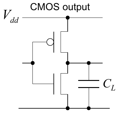
Lowering frequency alone does not remove leakage; longer runtime can increase static energy.
\(P_{dyn},P_{static},P_{total}\): dynamic, static, and total power [W]; \(\alpha\): switching activity; \(C_L\): load capacitance [F]; \(V_{dd}\): supply voltage [V]; \(f\): clock frequency [Hz]; \(I_{leak}\): leakage current [A]. Source: Chen Processing p.23; Marwedel (2021), Chapter 3.3.2.
Voltage/Frequency Scaling Example
Yasuura’s example relates voltage to maximum clock speed and energy per cycle.
| Supply | Maximum speed | Energy/cycle |
|---|---|---|
| 2.5 V | 25 MHz | 10 nJ |
| 5.0 V | 50 MHz | 40 nJ |
For equal cycle count, halving speed permits about one quarter of the dynamic energy in this example.
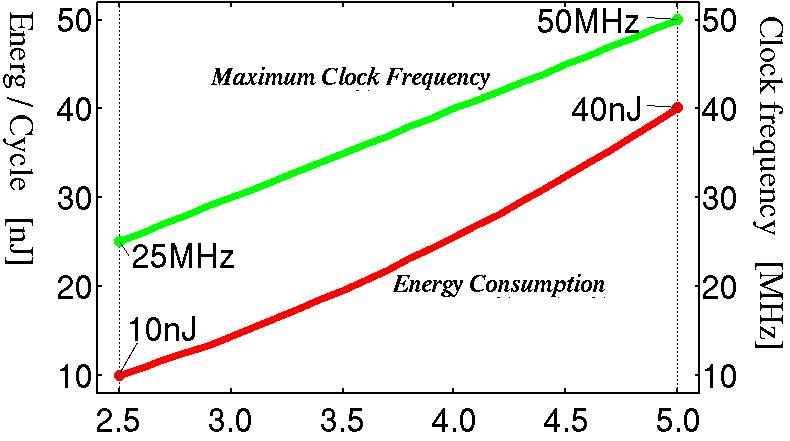
Use lower voltage only when timing permits; leakage and transition costs require separate accounting.
Yasuura 2000 via Chen Processing p.26.
Power Model: Frequency Dependence
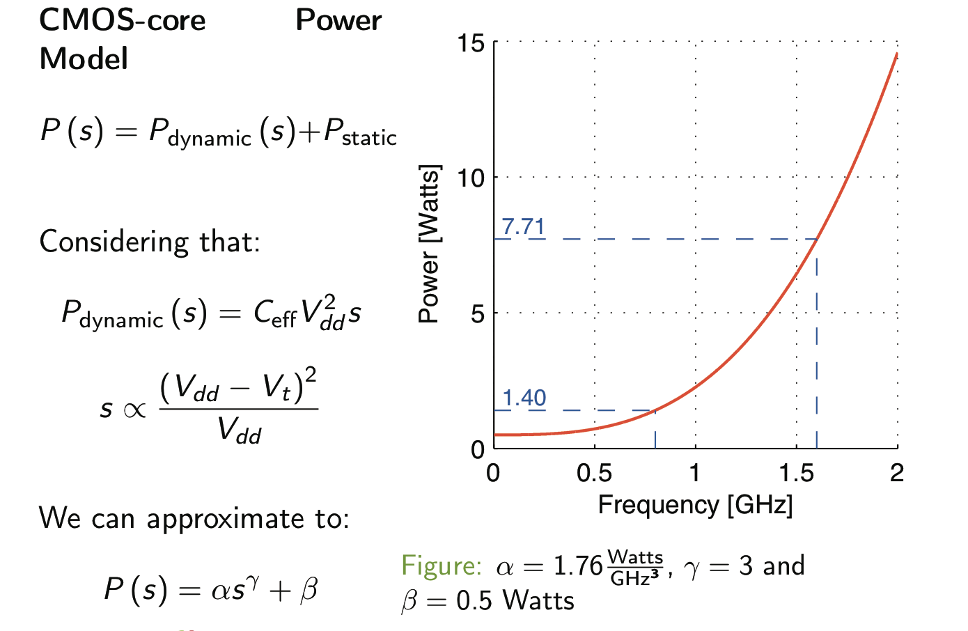
The graph shows core power \(P(s)\) as clock frequency \(s\) changes:
\[P(s)=\alpha s^\gamma+\beta\]
- Static power \(\beta=0.5\) W remains while the core is powered.
- With \(\gamma=3\), the dynamic term \(\alpha s^3\) grows steeply: voltage must rise to support higher clock speeds.
- Doubling \(s\) from 0.8 to 1.6 GHz raises total power \(P\) from 1.40 to 7.71 W, not merely by a factor of two.
Chen / Marwedel 2024, Processing, PDF p.27. \(s\): clock frequency; \(P(s)\): core power; \(\alpha\): fitted coefficient (not switching activity here); \(\gamma\): exponent; \(\beta\): static power. The frequency/voltage relation is approximated over the modeled operating range.
Energy Model: Critical Frequency
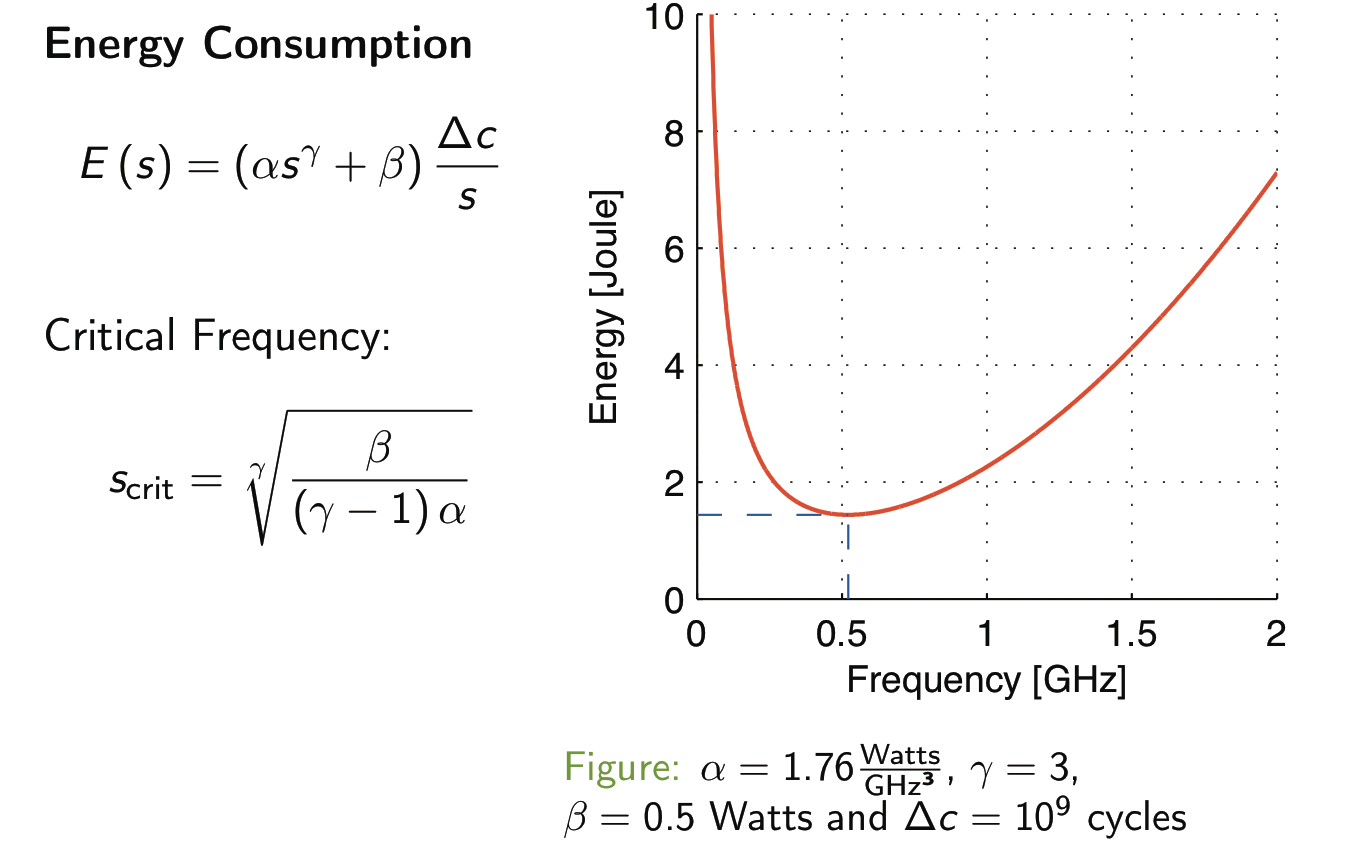
For the same work \(\Delta c=10^9\) cycles, task energy \(E(s)\) includes both power \(P(s)\) and execution time \(t=\Delta c/s\).
- High \(s\): the dynamic power term dominates; executing faster costs more energy \(E\).
- Low \(s\): longer runtime \(t\) increases leakage energy \(\beta t\).
- The minimum is near \(s_{crit}=0.52\) GHz, with \(E\approx1.44\) J. Slower is not always more efficient.
A deadline \(D\) also requires \(s\geq\Delta c/D\); the energy minimum may be too slow.
Chen / Marwedel 2024, Processing, PDF p.28. \(E(s)\): task energy; \(s\): clock frequency; \(\Delta c\): cycle count; \(\beta\): static power; \(s_{crit}\): energy-minimizing frequency. Same power-model parameters as on the preceding plot.
SA-1100: Power-State Automaton
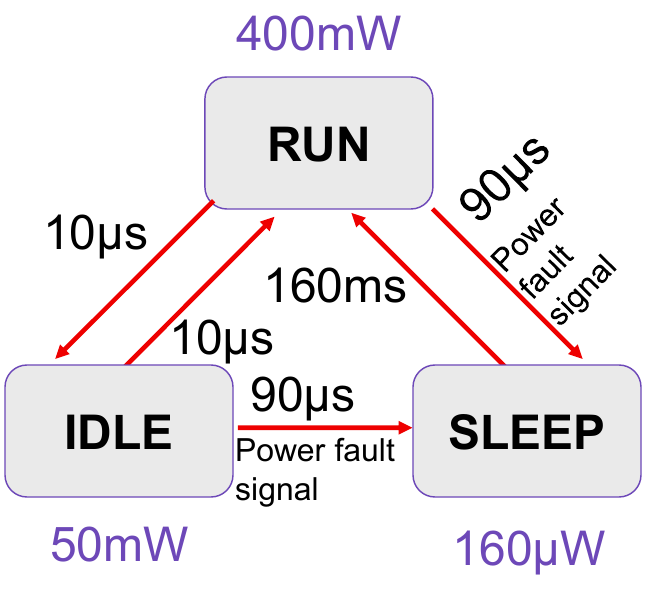
Chen / Marwedel 2024, Processing, PDF p.29.
Mobile Energy Budget
The ITRS 2010 projection compares component power \(P\) with a 0.5-1 W budget for small mobiles; larger mobiles were discussed around 7 W.
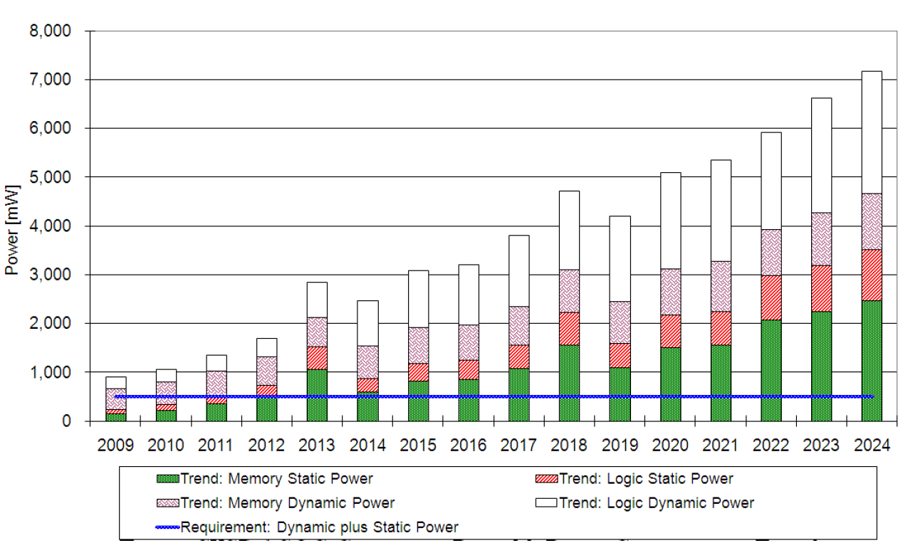
ITRS 2010 / Chen Processing p.31. Projection from 2010; processor, memory, radios, display and platform budget must be considered together.
Heterogeneous Processing and Power Gating
A heterogeneous SoC can combine specialized processing and independently powered domains.
In Chen’s W-CDMA example:
- Control and W-CDMA baseband are ON.
- GSM is mode-dependent; the application system domain is ON, its real-time domain OFF.
- Reported leakage: 407 microamperes, room temperature, 1.2 V.
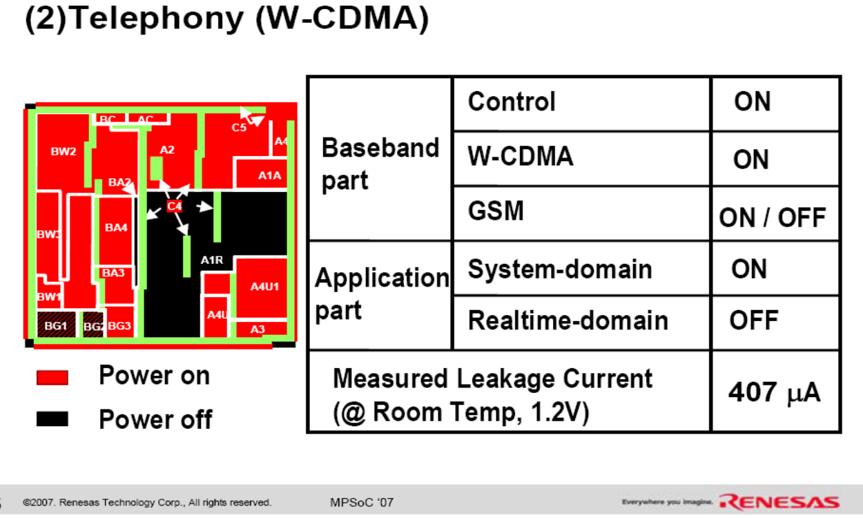
Power only the domains needed by the active use case.
Hattori / Renesas 2007; Chen Processing p.32.
big.LITTLE: Cortex-A15 and Cortex-A7 Pipelines
A complex Cortex-A15 provides higher peak performance; a simpler Cortex-A7 targets efficient execution at modest demand.
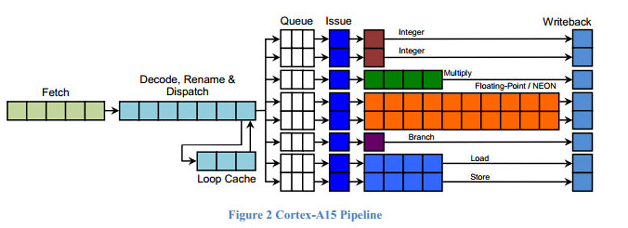
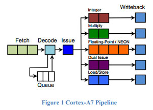
Left: Cortex-A15. Right: Cortex-A7.
ARM 2013; Chen Processing, PDF p.33.
big.LITTLE: Power and Performance
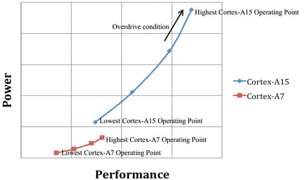
ARM 2013; Chen Processing, PDF p.33.
The scheduler must match workload phases to suitable cores while respecting latency and thermals. The example platform is Samsung Galaxy S4.